Linear Algebra, Linear Codes
In this section we will introduce linear codes, a type of error-correcting codes based on linear algebra over finite fields with conceptual and computational nice properties. We will start by reviewing linear algebra over finite fields, and especially paying attention to the null space of matrices. We will then define linear codes in terms of the null space of parity check matrices or the column space of the generator matrix. We will discuss the error-correction capabilities of linear codes and show how decoding is performed. Finally, we will introduce some common and important linear codes.
Linear algebra over finite fields
So far we have focused on vector spaces where the elements of vectors and matrices are real numbers. But digital codes live in discrete spaces. We need to work with vectors whose elements come from finite fields. The simplest case is binary vectors and matrices like:
\[A = \begin{pmatrix} \begin{matrix} 1 & 0 \\ 0 & 0 \\ 1 & 1 \\ \end{matrix} & \begin{matrix} 0 & 1 \\ 1 & 1 \\ 0 & 1 \\ \end{matrix} \\ \end{pmatrix},\qquad x = \left( 1,0,1,0 \right)\]Matrix algebra over finite field
Row space, column space, and null space
The row space, column space, and null space in a finite field \(\mathbb F\) are defined in the same way as matrices over real numbers. In particular, the row space is the span of the rows of the matrix, i.e., the set of all linear combinations of the rows of the matrix, where the coefficients are also from \(\mathbb F\) and all computations are performed in \(\mathbb F\). For example, consider
\[A=\begin{pmatrix}1&3&4\\2&2&3\end{pmatrix}\]in \(\mathbb F_5\). Then the following is a linear combination of the rows of \(A\):
\[\begin{pmatrix}3&2\end{pmatrix} \begin{pmatrix}1&3&4\\2&2&3\end{pmatrix}=3\begin{pmatrix}1&3&4\end{pmatrix}\oplus 2\begin{pmatrix}2&2&3\end{pmatrix}=\begin{pmatrix}3&4&2\end{pmatrix}\oplus \begin{pmatrix}4&4&1\end{pmatrix}=\begin{pmatrix}2&3&3\end{pmatrix}\]Note that multiplying a row vector from the left yields a linear combination of the rows and multiplying a column vector from the right yields a linear combination of the columns.
We can find the fundamental spaces similar to real matrices. To find the row space, we start by multiplying the first row by a scalar to make the first element of the first row into 1. Then we add appropriate scaled versions of the first row to the other rows to make their first element 0. Then we move to the second element of the second row and so on.
For example, a reduced basis for the row space of the matrix $B$
\[B = \begin{pmatrix}2&3&4\\2&2&3\end{pmatrix}\]is obtained as
where in the first step, we have replaced the first row by $3\times$ the first row. Note that part of the resulting matrix is the identity matrix. The rows of this matrix form a basis for the row spaces. So we can write the row space as
\[\left\{ \begin{pmatrix}x_1&x_2&3x_1+x_2\end{pmatrix}: x_1,x_2\in \mathbb F_4 \right\}.\]Unlike the spaces of matrices with real elements, spaces of finite field matrices are, well, finite. The row space above has in fact 25 vectors in it. These are listed below, where for brevity we have dropped the parentheses and spaces:
\[000,011,022,033,044,\\ 103,114,120,131,142,\\ 201,212,223,234,240,\\ 304,310,321,332,343,\\ 402,413,424,430,441.\]Now let us find the null space of this matrix. We can use the matrix obtained in \eqref{eq:rowBasis} to do so. But for our purpose, it is better to find a matrix which has the identity on its right side. To achieve this, we start from the last element of the last column and make it into a 1. Then we make the elements above this 1 into 0 and proceed backward:
\[\begin{pmatrix} 2 & 3 & 4\\ 2 & 2 & 3 \end{pmatrix}\xrightarrow{R_{2}\to2R_{2}} \begin{pmatrix} 2 & 3 & 4\\ 4 & 4 & \color{brown}{1} \end{pmatrix}\xrightarrow{R_{1}\to R_{1}+R_{2}} \begin{pmatrix} 1 & 2 & \color{brown}{0}\\ 4 & 4 & \color{brown}{1} \end{pmatrix}\xrightarrow{R_{1}\to3R_{1}} \begin{pmatrix} 3 & \color{brown}{1} & \color{brown}{0}\\ 4 & 4 & \color{brown}{1} \end{pmatrix}\xrightarrow{R_{2}\to R_{1}+R_{2}} \begin{pmatrix} 3 & \color{brown}{1} & \color{brown}{0}\\ 2 & \color{brown}{0} & \color{brown}{1} \end{pmatrix}\]The elements of the null space then satisfy
\[\begin{pmatrix} 3 & \color{brown}{1} & \color{brown}{0}\\ 2 & \color{brown}{0} & \color{brown}{1} \end{pmatrix} \begin{pmatrix}x_1\\\color{brown}{x_2}\\\color{brown}{x_3}\end{pmatrix}.\]We can write the elements that correspond to the identity part of the matrix in terms of the other ones:
\[x_2 = -3x_1 = 2x_1\\ x_3 = -2x_1 = 3x_1.\]So the null space is
\[NS(B) = \left\{\begin{pmatrix}x_1\\2x_1\\3x_1\end{pmatrix}:x_1\in\mathbb F_5\right\}=\{000,123,241,314,432\}.\]Finally, a generator for the null space is
\[G = \begin{pmatrix}1\\2\\3\end{pmatrix},\qquad NS(B) = \left\{G x_1: x_1 \in \mathbb F_5\right\}.\]Linear Codes
| Message | Codeword |
| 000 | 000000 |
| 100 | 100110 |
| 010 | 010101 |
| 001 | 001011 |
| 110 | 110011 |
| 101 | 101101 |
| 011 | 011110 |
| 111 | 111000 |
From linear equations to the parity-check matrix
Recall the binary code constructed as follows:
- Codeword: $\color{green}{x_{1}x_{2}x_{3}}\color{blue}{x_{4}x_{5}x_{6}}$
- Information bits: $\color{green}{x_{1}x_{2}x_{3}}$
- Parity bits:
The encoding table for this code is given on the right.
At the receiver, we check these three equations defining the parity bits. If they all hold, we declare that no error has occurred. But if at least one of these is not satisfied, we know an error has occurred. For example, suppose 101110 is received. Then
$1 = 1\oplus 0$ ✅
$1 \neq 1\oplus 1$ ❌
$0 \neq 0\oplus 1$ ❌
So we know an error has occurred, but which bit is erroneous?
Linear algebra will be helpful for answering this question.
Note that the set of equations defining this code can be written as
\[\begin{cases} \color{green}{x_{1}} \oplus \color{green}{x_{2}} \oplus \color{blue}{x_{4}} = 0 \\ \color{green}{x_{1}} \oplus \color{green}{x_{3}} \oplus \color{blue}{x_{5}} = 0 \\ \color{green}{x_{2}} \oplus \color{green}{x_{3}} \oplus \color{blue}{x_{6}} = 0 \\ \end{cases}\]We can write these as a matrix equation:
\[\begin{cases} \color{green}{x_{1}} \oplus \color{green}{x_{2}} \oplus \color{blue}{x_{4}} = 0 \\ \color{green}{x_{1}} \oplus \color{green}{x_{3}} \oplus \color{blue}{x_{5}} = 0 \\ \color{green}{x_{2}} \oplus \color{green}{x_{3}} \oplus \color{blue}{x_{6}} = 0 \\ \end{cases} \Longleftrightarrow \begin{pmatrix} \color{green}{1} & \color{green}{1} & 0 & \color{blue}{1} & 0 & 0 \\ \color{green}{1} & 0 & \color{green}{1} & 0 & \color{blue}{1} & 0 \\ 0 & \color{green}{1} & \color{green}{1} & 0 & 0 & \color{blue}{1} \\ \end{pmatrix} \begin{pmatrix} \color{green}{x_{1}} \\ \color{green}{x_{2}} \\ \begin{matrix} \color{green}{x_{3}} \\ \color{blue}{x_{4}} \\ \color{blue}{x_{5}} \\ \color{blue}{x_{6}} \\ \end{matrix} \\ \end{pmatrix} = 0\]We can thus define this code as the set of vectors $x$ such that $Hx = 0$, where
$H$ is called a parity check matrix. The code defined by $H$ is the vectors in its null space.
We can use $H$ to check the parity equations. For our previous example, in which 101110 was received,
\[H\begin{pmatrix}1\\0\\1\\1\\1\\0\end{pmatrix} = \begin{pmatrix}1\\1\\0 \end{pmatrix}\oplus \begin{pmatrix}0\\1\\1\end{pmatrix} \oplus \begin{pmatrix}1\\0\\0 \end{pmatrix}\oplus \begin{pmatrix}0\\1\\0\end{pmatrix} = \begin{pmatrix}0\\1\\1\end{pmatrix}.\]Since the answer is not $\mathbf 0$, an error has occurred. We will see later how the matrix $H$ can help us find which bit is erroneous. But for the moment, let us more closely study the codes defined in this way, which are called linear codes.
Why are the codes defined based on the null space of a matrix called linear codes? Because they satisfy the linear properties:
-
If $x$ and $y$ are codewords, then $x\oplus y$ is also a code word.
\[Hx=0,Hy=0\Rightarrow H(x\oplus y) = Hx\oplus Hy = 0.\] -
If $x$ is a codeword, then $ax$ is also a codeword for any $a\in \mathbb F$.
\[H(ax) = aHx = \mathbf 0.\]
For example, the codewords of the code defined by \eqref{eq:code1} is
\[C=\{000000,100110,010101,001011,110011,101101,011110,111000\}\]The sum of the the codewords, $010101$ and $001011$ is $011110$, which is another codeword.
Non-binary example:
Assuming \(x_i\in \mathbb F_3\), consider the code defined as
- Codeword: $\color{green}{x_{1}x_{2}}\color{blue}{x_3x_{4}}$
- Information bits: $\color{green}{x_{1}x_{2}}$
- Parity bits: \(\begin{cases} \color{blue}{x_{3}} = \color{green}{x_{1}} \oplus \color{green}{x_{2}} \\ \color{blue}{x_{4}} = \color{green}{x_{1}} \oplus 2\color{green}{x_{2}} \end{cases}\)
The parity check matrix is then
The parity check matrices given in \eqref{eq:code1H} and \eqref{eq:code2H} are of the form
\[H = \left( {\color{green}{A}}_{\left( {\color{green}{n}} - {\color{green}{k}} \right) \times {\color{green}{k}}} \middle| {\color{blue}{I}}_{\left( {\color{blue}{n}} - {\color{blue}{k}} \right) \times \left( {\color{blue}{n}} - {\color{blue}{k}} \right)} \right),\]which is called the systematic form, where
- $A$ is arbitrary and $I$ is the identity matrix
- $n$ is the length of the code
- $k$ is the number of message bits
- $n - k$ is the number of parity bits
As we will see in an example below, we can also define codes using parity check matrices that are not systematic. But the systematic form simplifies the encoding.
Unless otherwise stated, we assume the codes are binary and we work in $\mathbb F_2$.
As demonstrated by the next example, the parity check matrix doesn’t need to be necessarily of the form $(A\vert I)$. If it is not, we can make it so using elementary row operations, which do not alter the null space.
The generator matrix and encoding
Recall that a linear code is defined as the null space of a matrix $H$. We can also find a matrix $G$ such that the code is the column space of $G$. That is $G$ is a generator for the null space of $H$.
Example: consider the code with message bits $x_1,x_2,x_3$ and parity bits $x_4,x_5,x_6$ with the parity check matrix $H$,
\[H = \begin{pmatrix} \color{green}{1} & \color{green}{1} & 0 & \color{blue}{1} & 0 & 0 \\ \color{green}{1} & 0 & \color{green}{1} & 0 & \color{blue}{1} & 0 \\ 0 & \color{green}{1} & \color{green}{1} & 0 & 0 & \color{blue}{1} \\ \end{pmatrix} \Rightarrow \begin{cases} \color{green}{x_{1}} \oplus \color{green}{x_{2}} \oplus \color{blue}{x_{4}} = 0 \\ \color{green}{x_{1}} \oplus \color{green}{x_{3}} \oplus \color{blue}{x_{5}} = 0 \\ \color{green}{x_{2}} \oplus \color{green}{x_{3}} \oplus \color{blue}{x_{6}} = 0 \\ \end{cases}\]So the null space, i.e., the code, is the set of vectors of the form:
\[C = \left\{\ \begin{pmatrix} \color{green}{x_{1}} \\ \color{green}{x_{2}} \\ \color{green}{x_{3}} \\ \color{blue}{x_{1}} + \color{blue}{x_{2}} \\ \color{blue}{x_{1}} + \color{blue}{x_{3}} \\ \color{blue}{x_{2}} + \color{blue}{x_{3}} \\ \end{pmatrix} : x_1,x_2,x_3\in \mathbb F_2\right\}.\]But note that
\[\begin{pmatrix} \color{green}{x_{1}} \\ \color{green}{x_{2}} \\ \color{green}{x_{3}} \\ \color{blue}{x_{1}} + \color{blue}{x_{2}} \\ \color{blue}{x_{1}} + \color{blue}{x_{3}} \\ \color{blue}{x_{2}} + \color{blue}{x_{3}} \\ \end{pmatrix} = \begin{pmatrix} 1 \\ 0 \\ 0 \\ 1 \\ 1 \\ 0 \\ \end{pmatrix}x_{1} \oplus \begin{pmatrix} 0 \\ 1 \\ 0 \\ 1 \\ 0 \\ 1 \\ \end{pmatrix}x_{2} \oplus \begin{pmatrix} 0 \\ 0 \\ 1 \\ 0 \\ 1 \\ 1 \\ \end{pmatrix}x_{3} = \begin{pmatrix} 1 & 0 & 0 \\ 0 & 1 & 0 \\ 0 & 0 & 1 \\ 1 & 1 & 0 \\ 1 & 0 & 1 \\ 0 & 1 & 1 \\ \end{pmatrix}\begin{pmatrix} x_{1} \\ x_{2} \\ x_{3} \\ \end{pmatrix}.\]If we define $G$ as
\[G = \begin{pmatrix} \color{blue}{1} & 0 & 0 \\ 0 & \color{blue}{1} & 0 \\ 0 & 0 & \color{blue}{1} \\ \color{green}{1} & \color{green}{1} & 0 \\ \color{green}{1} & 0 & \color{green}{1} \\ 0 & \color{green}{1} & \color{green}{1} \\ \end{pmatrix},\]Then
\[C = \left\{G\begin{pmatrix} x_{1} \\ x_{2} \\ x_{3} \\ \end{pmatrix}: x_1,x_2,x_3\right\}.\]In fact, for every set of message bits $x_1,x_2,x_3$, the corresponding codeword is given by $Gx$. For example,
\[G\begin{pmatrix} 1 \\ 1 \\ 0 \\ \end{pmatrix} = \begin{pmatrix} 1 & 0 & 0 \\ 0 & 1 & 0 \\ 0 & 0 & 1 \\ 1 & 1 & 0 \\ 1 & 0 & 1 \\ 0 & 1 & 1 \\ \end{pmatrix}\begin{pmatrix} 1 \\ 1 \\ 0 \\ \end{pmatrix} = \begin{pmatrix} 1 \\ 0 \\ 0 \\ 1 \\ 1 \\ 0 \\ \end{pmatrix} \oplus \begin{pmatrix} 0 \\ 1 \\ 0 \\ 1 \\ 0 \\ 1 \\ \end{pmatrix} = \begin{pmatrix} 1 \\ 1 \\ 0 \\ 0 \\ 1 \\ 1 \\ \end{pmatrix}\]A linear code over $\mathbb{F}_{3}$
Let $H$ be the parity check matrix of a code in $\mathbb F_3$,
\[H = \begin{pmatrix} 1 & 1 & 1 & 0 \\ 1 & 2 & 0 & 1 \\ \end{pmatrix}.\]The null space:
\[\begin{pmatrix} 1 & 1 & 1 & 0 \\ 1 & 2 & 0 & 1 \\ \end{pmatrix} \rightarrow \begin{pmatrix} x_{1} \\ x_{2} \\ -x_{1} - x_{2} \\ -x_{1} - 2x_{2} \\ \end{pmatrix} = \begin{pmatrix} x_{1} \\ x_{2} \\ 2x_{1} + 2x_{2} \\ 2x_{1} + x_{2} \\ \end{pmatrix} = \begin{pmatrix} \begin{matrix} 1 \\ 0 \\ 2 \\ 2 \\ \end{matrix} & \begin{matrix} 0 \\ 1 \\ 2 \\ 1 \\ \end{matrix} \\ \end{pmatrix}\begin{pmatrix} x_{1} \\ x_{2} \\ \end{pmatrix} \Rightarrow G = \begin{pmatrix} \begin{matrix} 1 \\ 0 \\ 2 \\ 2 \\ \end{matrix} & \begin{matrix} 0 \\ 1 \\ 2 \\ 1 \\ \end{matrix} \\ \end{pmatrix}\]Example codeword = \(G\begin{pmatrix} 1 \\ 2 \\ \end{pmatrix} = \begin{pmatrix} 1 \\ 2 \\ 0 \\ 1 \\ \end{pmatrix}\)
Properties of linear codes
- $x$ is a codeword if and only if $Hx = 0$
- If $H$ is of the systematic form $$H_{(n-k)\times n} = \left( {\color{green}{A}}_{\left( {\color{green}{n}} - {\color{green}{k}} \right) \times {\color{green}{k}}} \middle| {\color{blue}{I}}_{\left( {\color{blue}{n}} - {\color{blue}{k}} \right) \times \left( {\color{blue}{n}} - {\color{blue}{k}} \right)} \right),$$ then the codewords look like $$x = \color{green}{\underset{message}{\underbrace{x_{1}\cdots x_{k}}}}\color{blue}{\underset{parity}{\underbrace{x_{k + 1}\cdots x_{n}}}},$$ where $n$ is the length of the code and $k$ is the number of its message bits. $k$ is also called the dimension of the code as it is the dimension of the null space.
- When $H$ has the systematic form above, we can find a generator matrix $G$, $$G_{n\times k} = \left(\begin{array}{c} I_{k}\\ -A_{\left(n-k\right)\times k} \end{array}\right)$$ and encoding can be performed by $$\begin{pmatrix}\color{green}{x_1\\\vdots\\x_k}\\\color{blue}{x_{k+1}\\\vdots\\ x_n}\end{pmatrix} = G \begin{pmatrix}\color{green}{x_1\\ \vdots \\ x_k}\end{pmatrix}.$$
- Linear codes can be defined over any finite field (not limited to $\mathbb{F}_{2}$)
- Linearity: if $x$ and $y$ are codewords, then $ax$, $x \oplus y$, and $x \ominus y$ are also codewords
When $H$ is not in systematic form, if it is of size $\left( n - k \right) \times n$ and has $n - k$ linearly independent rows, then there are $k$ message bits and $n - k$ parity bits, each resulting from one row of $H$.
Minimum distance of linear codes
Recall: Hamming distance is the number of positions in which two codewords are different \(d_{H}\left( \mathbf{1}0\mathbf{0}11,\mathbf{0}0\mathbf{1}11 \right) = 2\).
Definition: Hamming weight of a codeword is the number of its nonzero elements \(w_{H}\left( 10011 \right) = 3\).
What is the relationship between the two? $d_{H}\left( x, y \right) = w_{H}\left( x \ominus y \right)$. Note that for binary $x \ominus y = x \oplus y$.
Recall: The minimum distance of a code is the smallest distance between two codewords
Do we need to compute the distance between every pair of codewords? No!
Proof: Suppose $x,y$ have the smallest distance. Then, $d_{H}\left( x,y \right) = w_{H}(x \ominus y)$. But $x \ominus y$ is a codeword. So there is a codeword whose weight is the minimum distance. On the other hand, no codeword can have a weight less than the minimum distance because the weight of each codeword is equal to its distance from the codeword 00…0.
We can also find the minimum distance directly from $H$, based on the following observation: If there is a codeword of weight $d$, then there are $d$ columns whose linear combination can produce $\mathbf 0$. So the minimum distance is the smallest number $d$ such that there are $d$ columns in $H$ whose linear combination can produce $\mathbf 0$.
- The only way that $d=1$ can occur is to have an all-0 column in $H$.
- Assuming $d>1$, for $d=2$, we need one column to be a mulitple of another column.
- In binary, we need two equal columns. So if all columns are distinct, then $d>2$.
- Assuming $d>2$, for $d=3$, we need three columns that are linearly dependant.
- In binary, the sum of two columns must be equal to a third column.
For the matrix $H$ of the previous exercise:
- No column is all-0 $\Rightarrow d > 1$
- No two columns are equal $\Rightarrow d > 2$
- Adding columns 1, 2, and 3 gives 0 $\Rightarrow d = 3$.
What is the relationship between minimum distance and rank of $H$?
- If the rank is $r$, then there are $r$ linearly independent columns
- If the minimum distance is $d$, every $d - 1$ columns are linearly independent
- Hence, $r \geq d - 1$ and so $d\le r+1$.
For the previous exercise, min distance is 3 and rank is also 3.
If the parity check matrix has dimensions $(n-k)\times n$, i.e., there are $n-k$ parity bits, then its rank is at most $n-k$ (why?). Hence, we find the following bound on the minimum distance of code:
Correcting erasure errors: solving equations
If the minimum distance of a code is $d$, then it can correct up to $d-1$ erasure errors. We can find the erased values by solving the equation $Hx=\mathbf 0$.
As an example consider the code given by the parity check matrix
\[H = \begin{pmatrix} 1 & 1 & 0 & 1 & 0 & 0 \\ 1 & 0 & 1 & 0 & 1 & 0 \\ 0 & 1 & 1 & 0 & 0 & 1 \end{pmatrix}.\]This code has minimum distance 3. So we can correct up to 2 erasures. Suppose that $x=100110$ is transmitted. We will look at some cases in which some of the bits are erased during transmission:
- Suppose that the second bit is erased, i.e., $1?0110$ is received. To find it, we can solve the equation: $$H\begin{pmatrix}1\\x_2\\0\\1\\1\\0\end{pmatrix}=\mathbf 0\Rightarrow \begin{pmatrix}1\\1\\0\end{pmatrix}\oplus x_2\begin{pmatrix}1\\0\\1\end{pmatrix} \oplus \begin{pmatrix}1\\0\\0\end{pmatrix} \oplus \begin{pmatrix}0\\1\\0\end{pmatrix}=\mathbf 0 \Rightarrow x_2\begin{pmatrix}1\\0\\1\end{pmatrix} =\mathbf 0 \Rightarrow x_2 = 0.$$ We had three eqeuations and one unknown, which we could solve.
- Suppose that the first and second bits are erased, i.e., $??0110$ is received. To find them, we can solve the equation: $$H\begin{pmatrix}x_1\\x_2\\0\\1\\1\\0\end{pmatrix}=\mathbf 0\Rightarrow x_1\begin{pmatrix}1\\1\\0\end{pmatrix}\oplus x_2\begin{pmatrix}1\\0\\1\end{pmatrix} \oplus \begin{pmatrix}1\\0\\0\end{pmatrix} \oplus \begin{pmatrix}0\\1\\0\end{pmatrix}=\mathbf 0 \Rightarrow x_1\begin{pmatrix}1\\1\\0\end{pmatrix}\oplus x_2\begin{pmatrix}1\\0\\1\end{pmatrix} = \begin{pmatrix}1\\1\\0\end{pmatrix} \Rightarrow \begin{cases}x_1\oplus x_2 = 1\\ x_1=1\\ x_2 = 0\end{cases}$$
- Suppose that the first, second, and third bits are erased, i.e., $???110$ is received. To find them, we can solve the equation: $$H\begin{pmatrix}x_1\\x_2\\x_3\\1\\1\\0\end{pmatrix}=\mathbf 0\Rightarrow x_1\begin{pmatrix}1\\1\\0\end{pmatrix}\oplus x_2\begin{pmatrix}1\\0\\1\end{pmatrix}\oplus x_3\begin{pmatrix}0\\1\\1\end{pmatrix} \oplus \begin{pmatrix}1\\0\\0\end{pmatrix} \oplus \begin{pmatrix}0\\1\\0\end{pmatrix}=\mathbf 0 \Rightarrow x_1\begin{pmatrix}1\\1\\0\end{pmatrix}\oplus x_2\begin{pmatrix}1\\0\\1\end{pmatrix}\oplus x_3\begin{pmatrix}0\\1\\1\end{pmatrix} =\begin{pmatrix}1\\1\\0\end{pmatrix} \Rightarrow \begin{cases}x_1\oplus x_2 = 1\\ x_1\oplus x_3=1\\ x_2\oplus x_3 = 0\end{cases}$$ While we have three equations and three unknowns, the third equation is the sum of the other two. So we have in fact two equations, which is not sufficient to determine the codeword reliably. There are two possibilities: 100110, 011110.
Correcting substitution errors: syndrome decoding
Suppose we receive a word $y$ at the receiver (or read it from a flash drive). We know that there may have been errors. Assuming that the number of errors are less than half of the minimum distance, we should be able to correct them and find the transmitted codeword $x$. But how? This is the decoding problem.
It will be helpful to think of errors as adding a vector $e$ to $x$. The output is $y = x + e$.
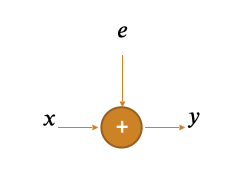
Example:
- $x$ = 10001001
- $e$ = 00010000
- $y$ = 10011001
The number of errors equals to the weight of $e$.
At the receiver, we only know $y$ but don’t know what $e$ and $x$ are.
Parity check equations
The parity check equations are key to finding whether or not there are any errors and finding them. As an example, consider the code defined by the following parity check matrix:
We receive $y = \text{101011}$. Is there any error? If so, what was sent?
We know that if there are no errors, then $y$ is equal to $x$ and satisfies the parity equations. So we check to see if the parity equations are satisfied for $y$:
- $y_{1} + y_{2} + y_{4} = 1 + 0 + 0 = 1 \neq 0$ ❌
- $y_{1} + y_{3} + y_{5} = 1 + 1 + 1 = 1 \neq 0$ ❌
- $y_{2} + y_{3} + y_{6} = 0 + 1 + 1 = 0$ ✅
This indicates that there was at least one error. But which bit(s) is/are incorrect?
Recall that each row of the parity check matrix corresponds to one parity equation. We can check all parity equations with matrix algebra by finding $s = Hy$. This is called the syndrome.
\[s = Hy = \begin{pmatrix} 1 & 1 & 0 & 1 & 0 & 0 \\ 1 & 0 & 1 & 0 & 1 & 0 \\ 0 & 1 & 1 & 0 & 0 & 1 \\ \end{pmatrix}\begin{pmatrix} 1 \\ 0 \\ 1 \\ 0 \\ 1 \\ 1 \\ \end{pmatrix} = \begin{pmatrix} 1 \\ 1 \\ 0 \\ \end{pmatrix} + \begin{pmatrix} 0 \\ 1 \\ 1 \\ \end{pmatrix} + \begin{pmatrix} 0 \\ 1 \\ 0 \\ \end{pmatrix} + \begin{pmatrix} 0 \\ 0 \\ 1 \\ \end{pmatrix} = \begin{pmatrix} 1 \\ 1 \\ 0 \\ \end{pmatrix}\]The first and second elements are nonzero, indicating first and second equations are not satisfied.
So if the syndrome is nonzero, we know that there are errors. But the syndrome can also help us to find which bits are incorrect. Recall that $y=x+e$. So
\[s = Hy = H\left( x + e \right) = Hx + He = He.\]We thus have the equation $s=He$.
If we can solve this equation, we can find $e$ and thus $x$.
For this example, we must solve this equation for $e$
\[He = s \Rightarrow \begin{pmatrix} 1 & 1 & 0 & 1 & 0 & 0 \\ 1 & 0 & 1 & 0 & 1 & 0 \\ 0 & 1 & 1 & 0 & 0 & 1 \\ \end{pmatrix}e = \begin{pmatrix} 1 \\ 1 \\ 0 \\ \end{pmatrix}\]But how can we solve this equation? Is there a unique solution? To find out how to solve this, let’s first see a couple of examples with known $e$.
- $e_1 = 010000.$
- $e_2 = 000100.$
- $e_3 = 010001.$
Based on the previous exercise, we make the following observations:
- The syndrome is equal to the sum of the columns of $H$ where the errors occurred.
- Multiple error vectors, perhaps with different number of errors in each, can lead to the same syndrome.
Back to the equation:
\[\begin{pmatrix} 1 & 1 & 0 & 1 & 0 & 0 \\ 1 & 0 & 1 & 0 & 1 & 0 \\ 0 & 1 & 1 & 0 & 0 & 1 \\ \end{pmatrix}e = \begin{pmatrix} 1 \\ 1 \\ 0 \\ \end{pmatrix}\]The obvious solution is $e=100000$, indicating an error in the first bit: $x = y - e = 101011 - 100000 = 001011$.
There are other solutions, but they all indicate more than one error: 011000, 000110,…. For example, if $x = 110011$ and $e = 011000$, then $y = 101011$ and we get the same syndrome. If the probability of error is small, $e = 100000$ is more likely than $e = 011000$.
- What is the probability of the following error vectors?
- $e_1 = 100000$
- $e_2 = 011000$
- $e_3 = 000110$
- If the probability $q$ of bit flip errors is small, we can use the approximation $1-q \simeq 1$. Using this approximation find the probability of each error vector.
- Let $q=10^{-6}$ and find the numerical values of the probabilities of the error vectors, both using the exact expressions and the approximations.
Example: Same $H$ but with $y =$100110.
The syndrome is
\[s = \begin{pmatrix} 1&1&0&1&0&0 \\ 1&0&1&0&1&0 \\ 0&1&1&0&0&1 \\ \end{pmatrix}y = \begin{pmatrix} 0 \\ 0 \\ 0 \\ \end{pmatrix}\Rightarrow\begin{pmatrix} 1&1&0&1&0&0 \\ 1&0&1&0&1&0 \\ 0&1&1&0&0&1 \\ \end{pmatrix}e = \begin{pmatrix} 0 \\ 0 \\ 0 \\ \end{pmatrix}.\]We declare no error, since $e = 000000$ is a solution. Could there be an undetected error? Yes, for example, if $x = \text{01111}\text{0}$ and $e = 111000$, then $y = 100110$ and $s = Hy = 0$. But if the probability of error is small, $e = 111000$ is far more unlikely than $e = 000000$.
Syndrome decoding summary:
- Compute $s = Hy$
- If $s = 0$, declare no error!
- If $s \neq 0$, solve $He = s$ for $e$. There will be many possible solutions; we find the one with the smallest weight (smallest number of errors, most likely case).
- Find $x = y \ominus e$
- $y_1 = 100110$.
- $y_2 = 110111$
- $y_3 = 100001$
- $y_4 = 001010$
- Pick a sequence of three bits as a message to be transmitted. Let these bits be denoted by $x_1x_2x_3$.
- Encode the message $x_1x_2x_3$ using the generator matrix given below: $$x = \begin{pmatrix} x_{1} \\ x_{2} \\ x_{3} \\ x_{4} \\ x_{5} \\ x_{6} \\ \end{pmatrix} = G\begin{pmatrix} x_{1} \\ x_{2} \\ x_{3} \\ \end{pmatrix},\qquad G = \begin{pmatrix} 1 & 0 & 0 \\ 0 & 1 & 0 \\ 0 & 0 & 1 \\ 1 & 1 & 0 \\ 1 & 0 & 1 \\ 0 & 1 & 1 \\ \end{pmatrix}$$ Call the resulting codeword $x$.
-
Assume $x$ is transmitted through a noisy channel. Pick three different error vectors with
- $e_1$, with 1 error
- $e_2$, with 2 errors
- $e_3$, with 3 errors
- Using the provided parity check matrix, decode $y_1,y_2,y_3$, assuming the smallest number of errors that give the received word. $$H = \begin{pmatrix} 1 & 1 & 0 & 1 & 0 & 0 \\ 1 & 0 & 1 & 0 & 1 & 0 \\ 0 & 1 & 1 & 0 & 0 & 1 \\ \end{pmatrix}$$ In which cases was the decoding successful?
Correcting 1 error: Hamming Codes
Suppose our goal is to correct 1 error. What property should the parity check matrix have? We require minimum distance of at least 3, which means no two vectors should be linearly dependent. For binary, it suffices to not have the all-0 column and also for all columns to be distinct. Another way to arrive at the same conclusion is to note that we must always be able to solve the equation
\[s=He\]as long as $e$ has at most a single 1. Remember that if only the $j$th position in $e$ is 1, then $He$ is equal to the $j$th column of $H$. To be able to find $j$, the columns of $H$ must be distinct. Also, the columns must be non-zero to be able to distinguish no error from 1 error.
Let’s construct such a parity check matrix when there are three parity bits ($H$ has three rows). There are 7 columns with 3 bits in them. So $H$ must have these 7 columns. We arrange them in the systematic form.
\[H = \begin{pmatrix} 1 & 1 & 0 & 1 & 1 & 0 & 0 \\ 1 & 0 & 1 & 1 & 0 & 1 & 0 \\ 0 & 1 & 1 & 1 & 0 & 0 & 1 \\ \end{pmatrix}\]What is the minimum distance?
- $d \geq 3$, since all columns are distinct and nonzero.
- $d \leq 3$, since $x = 1110000$ is a codeword
- Hence, $d = 3$
What are the parity check equations?
This is the [7,4,3]-Hamming code: it has length $n = 7$, it has $k = 4$ message bits, and its minimum distance is $d = 3$. There are other Hamming codes based on the same idea as we will see. We sometimes drop the minimum distance from this notation.
Possible codewords of the [7,4]-Hamming code are:
0000000 0001111 0110110 1011010
1000110 1100011 0101010 1101100
0100101 1010101 0011100 1110000
0010011 1001001 0111001 1111111
| Message | Bits | Message | Bits | |
|---|---|---|---|---|
| 🐙 | 0000000 | 🐘 | 0001111 | |
| 🐉 | 0010011 | 🐋 | 0011100 | |
| 🐒 | 0100101 | 🐕 | 0101010 | |
| 🐧 | 0110110 | 🦁 | 0111001 | |
| 🦏 | 1000110 | 🦒 | 1001001 | |
| 🦓 | 1010101 | 🦖 | 1011010 | |
| 🦅 | 1100011 | 🦋 | 1101100 | |
| 🦉 | 1110000 | 🐥 | 1111111 |
Alter the keyword by applying 1 error, 2 errors, and 3 errors to produce three received vectors. Enter the received vectors below and click the "Decode" button, to correct the errors using a decoder that can correct at most one error. In which cases was the error detected and in which cases it wasn't?
We can extend the idea of the $[7,4]$-Hamming code to design longer codes if we use more parity bits. If we have $r$ parity bits, i.e., $H$ has $r$ rows, then there are $2^r-1$ possible nonzero columns. So we can construct a parity check matrix with $2^r-1$ columns and $r$ rows. So the length of the code is $n=2^r-1$ bits. Among these, $r$ are parity bits and the rest are message bits. This results in the $[2^r-1,2^r-r-1]$-Hamming code. This code still has minimum distance 3.
Example: [15,11,3]-Hamming code:
\[H = \begin{pmatrix} 1 & 1 & 1 & 0 & 0 & 0 & 1 & 1 & 1 & 0 & 1 & 1 & 0 & 0 & 0 \\ 1 & 0 & 0 & 1 & 1 & 0 & 1 & 1 & 0 & 1 & 1 & 0 & 1 & 0 & 0 \\ 0 & 1 & 0 & 1 & 0 & 1 & 1 & 0 & 1 & 1 & 1 & 0 & 0 & 1 & 0 \\ 0 & 0 & 1 & 0 & 1 & 1 & 0 & 1 & 1 & 1 & 1 & 0 & 0 & 0 & 1 \\ \end{pmatrix}\]Let’s consider which code is better, the $[7,4]$-Hamming code or the $[15,11]$-Hamming code? The two main properties of codes are the code rate and the error-correction capability.
Code rate: The code rates for these codes are $\frac47=0.57$ and $\frac{11}{15}=0.73.$ So the $[15,11]$-Hamming code has a higher rate (less overhead), which is better.
Error-correction: They are both guaranteed to correct up to 1 error. So it may seem that overall the $[15,11]$-code is better. But this code is also longer, increasing the probability of more than 1 error. To see this, suppose the probability of a single bit flip is $q=10^{-6}$. What is the probability of at least 2 errors in a codeword for each of the codes? For the $[7,4]$ code, the probability of at least 2 errors is
\[1-\left((1-q)^7+\binom71(1-q)^6q\right)=1-(1-q)^6(1+6q)=2.09999\times 10^{-11}\]and for the $[15,11]$-code
\[1-\left((1-q)^{15}+\binom{15}1(1-q)^{14}q\right)=1-(1-q)^{14}(1+14q)=1.04999\times 10^{-10}.\]So the longer code is 5 times as likely to suffer from an undetected error. There is no clear winner; which one we choose depends on the application.
Correcting multiple errors
How can we correct multiple errors with a linear code?
For two errors, we need minimum distance of 5. So every set of 4 columns must be linearly independent. An example of such a parity check matrix is
\[H = \begin{pmatrix} 1 & 1 & 0 & 0 & 0 \\ 1 & 0 & 1 & 0 & 0 \\ 1 & 0 & 0 & 1 & 0 \\ 1 & 0 & 0 & 0 & 1 \\ \end{pmatrix}\]But the rate is very small: $\frac15$. Codes with better rates can be obtained based on finite fields of size $2^{m}$, $m>1$, which have more complex structures. An example is given below. (This is a BCH code.)
\[H = \begin{pmatrix} 1&0&0&0&1&0&0&1&1&0&1&0&1&1&1 \\ 0&1&0&0&1&1&0&1&0&1&1&1&1&0&0 \\ 0&0&1&0&0&1&1&0&1&0&1&1&1&1&0 \\ 0&0&0&1&0&0&1&1&0&1&0&1&1&1&1 \\ 1&0&0&0&1&1&0&0&0&1&1&0&0&0&1 \\ 0&0&0&1&1&0&0&0&1&1&0&0&0&1&1 \\ 0&0&1&0&1&0&0&1&0&1&0&0&1&0&1 \\ 0&1&1&1&1&0&1&1&1&1&0&1&1&1&1 \\ \end{pmatrix}\]MDS codes
Let us consider first how codes can be used for data storage to protect against hard drive failure. Suppose that we have a code with length $n$, with $k$ information bits, and with minimum Hamming distance $d$. We can put one bit from each codeword on each hard drive. For example, suppose the code is defined by
\[\color{blue}{x_4} = \color{green}{x_1}\oplus \color{green}{x_2} \oplus \color{green}{x_3},\]where $n=4,k=3$ and $x_1x_2x_3$ are message bits and $x_4$ is the only parity bit. We can write $x_1$ on drive 1, $x_2$ on drive 2 and so on, and do the same for the next codeword:
Drive 1: $\color{green}{1000101001}\dotsc$
Drive 2: $\color{green}{1001010100}\dotsc$
Drive 3: $\color{green}{0111101110}\dotsc$
Drive 4: $\color{blue}{0110010011}\dotsc$
For example, the first bit on drive 4 is the parity bit for the first bits on the other drives. In this way, if any single drive fails, we can reconstruct its data. Note that hard drive failures are erasures since data is lost and we know which bits are affected (as opposed to substitution errors). For example, if the second drive fails, we can recover its data using
\[x_2 = x_1+x_3+x_4.\]MDS Codes: Recall that for a code of length $n$ and dimension $k$, the Singleton bound says
\[d \leq n - k + 1.\]Codes that achieve the Singleton bound are called maximum distance separable (MDS). That is for MDS codes,
\[d = n - k + 1.\]These codes are very common in data storage. Recall that if the minimum distance is $d$, then we can correct $d-1$ erasure errors. For MDS codes, we can correct $n-k$ erasures. So, if we have $k$ hard drives worth of data to store, we can use an MDS code and write the data on $n$ drives, where $n>k$. Then even if some drives fail, as long as $k$ are still operational, we can recover our data! A well-known family of MDS codes are Reed-Solomon codes.
Back to the data center
Let’s look at some of the ways we could protect data stored in a data center, like the Facebook data center we mentioned in the beginning of this chapter:
- Replication with two copies (triple redundancy).
- Single Parity: group hard drives into sets of 6 drives. Add a 7th drive that stores the parity bits. If any drive is lost, we can recover its data.
- [7,4]-Hamming code. If up to two drives from the set of 7 drives are lost, we can recover the data.
- Reed-Solomon code: $k$ data drives and $r$ parity drives. Data can be recovered from any $k$ drives.
In the Facebook warehouse, frequently accessed data is protected by replication and less frequently accessed data uses Reed-Solomon with $k = 10,r = 4$.
- 40% more storage used
- Out of a group of 14 drives, if any 4 fail, we won’t lose any data.