Frequency and Spectrum

A signal is a function of time $x(t)$ in audio, or a function of space $I(x, y)$ in an image.

Another way to describe a signal is by the frequency content.

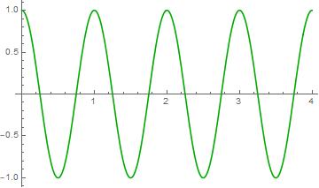
Let us start by imagining a single sinusoid (a cosine function or a sine function, for example): $x(t) = A \cos(2 \pi f t + \phi)$

This sinusoid has three parameters: the amplitude A, the frequency f, and the phase φ. The period is the smallest time T such that $x(t) = x(t + T)$ for all t. The following interactive graph may help you understand these concepts.

What is frequency?

In the sinusoid example, the frequency f is the inverse of the period T. The faster the signal repeats, the higher its frequency.

So the frequency measures how fast a single tone repeats.

Yes, but it can be used in other contexts as well, even when the signal is not periodic…

Sound waves and music

Sound and music are good ways to better understand frequencies. Music generally consists of chords that contain multiple notes simultaneously.

Play

What are the units of frequency?

Generally speaking, frequency is measured in cycles/unit time.

When time t is in seconds, frequency f is in cycles/second, or Hertz (Hz).

Music generally measures notes relative to “high A”, which has a frequency of 440 Hz.

How fast is 440 Hz?

We can also measure frequency in radians/unit time. This measure of frequency, $ω = 2πf$, is commonly encountered when describing the behavior of analog electronic circuits.

440 Hz = 2764.6 radians/second

We are used to describing many kinds of signals in terms of their frequency content.

Light (frequency = color)

Radio (frequency = station)

Music (frequency = note)

Video (frequency = frame rate)

Heart beat (frequency = heart rate)

Brain waves (frequency = alpha/beta/gamma/…)

Light and frequency

Visible light exists in many colors. These colors reflect the frequency, or equivalently the wavelength, of the light wave: wavelength (λ) = speed of light (c) / frequency (ν)

Violet light has the highest frequency (670-790 THz), and the shortest wavelength (380-450 nm).

Next comes blue light (600-670 THz), then green (520-600 THz), yellow (510-520 THz), orange (480-510 THz), and finally red light (400-480 THz).

The energy (E) of the corresponding light photon increases with increasing frequency: $E = h \nu = \frac{h c}{\lambda}$. h = Planck’s constant ($6.6 \times 10^{-34} J\cdot s)$.

In fact, how we perceive visible light is due to its frequency:

The back of the eye (retina) contains two types of light-sensitive cells: rods and cones.

Rods are sensitive to a wide range of light frequencies.

Cones are sensitive to particular ranges of frequencies corresponding roughly to blue, green, and red.

The optic nerve transmits signals from these cells to the brain, which synthesizes them into colors.

Cameras and colors

1855: The idea of three color-sensitive cone cells was posited by James Clerk Maxwell (yes, that Maxwell) as a possible basis for color photography.

1868: Louis du Hauron patented the basic process for producing color photographs on paper. This idea is based on subtractive color, i.e., forming colors by removing components of white light (that contains all colors). This is also how color printers work, with cyan, magenta, and yellow ink instead of red, green, and blue.

1935: Eastman Kodak introduced color camera film (Kodachrome), with three layers of emulsion that recorded the red, green, and blue components of light. Agfa developed improved film a year later, that would allow developing all three colors simultaneously.

1963: Polaroid introduced color film for their instant camera.

Digital cameras work similarly:

Silicon-based sensors convert incident photons into energy, read out as voltages.

Filters placed on these sensors make them sensitive to specific ranges of light.

Cameras can arrange these sensors in an alternating mosaic like the Bayer pattern on the right. Image demosaicking takes the red, green, and blue images and aligns them to form a single RGB color image.

Some modern cameras can stack these sensors and filters to get red, green, and blue together.

Other electromagnetic radiation is also characterized by its frequency:

Ultraviolet (7.5×10^14 – 3×10^16 Hz)

Infrared (3×10^11 – 4.3×10^14 Hz)

X-rays (3×10^16 – 3×10^19 Hz)

Gamma rays (> 3×10^19 Hz)

Microwaves (3×10^8 – 3×10^11 Hz)

Radio waves (30 – 3×10^8 Hz)

Energy increases as frequency increases – this is why ultraviolet radiation can cause skin cancer, and repeated, significant X-ray or gamma radiation exposure can be deadly.

Fortunately, extremely high energy radiation from the sun is mostly disrupted by the earth’s magnetic field and the ozone layer. Or we’d all be cooked like a rotisserie chicken!

Sound waves and music

Like light, sound propagates as a wave, and hence can be described as a sinusoid (or a collection of sinusoids).

Humans can hear sounds with frequencies between 20 – 20,000 Hz (this varies with age, and person-to-person)

Dogs can hear up to nearly 50,000 Hz!

Dolphins can hear up to 150,000 Hz!!!

Pure sinusoids are called tones. These have single frequencies.

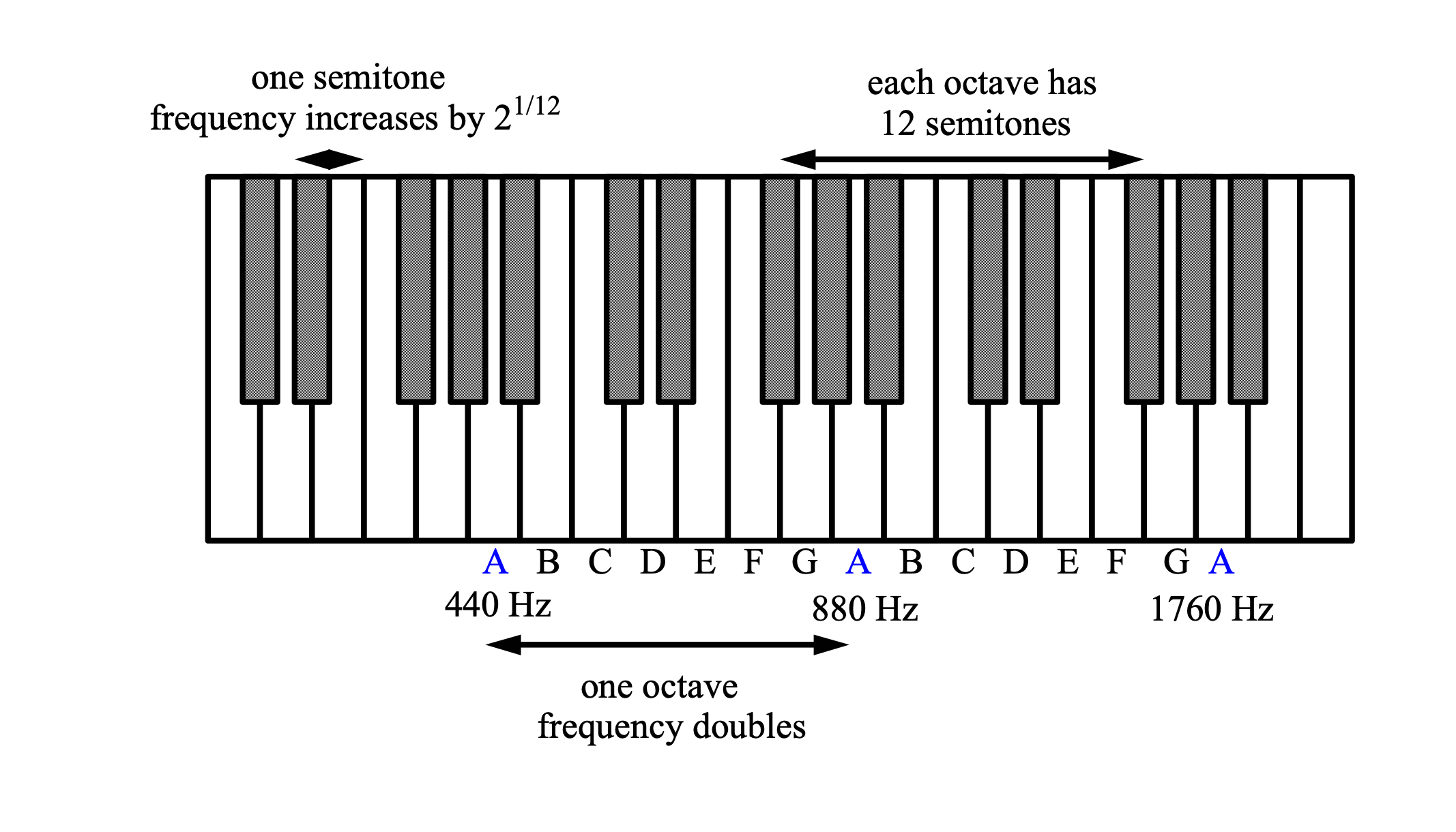
High “A” = 440 Hz

Middle “C” = 262 Hz

Each octave corresponds to doubling in frequency.

Actual musical notes are more complicated. Music generally consists of chords that contain multiple notes simultaneously.

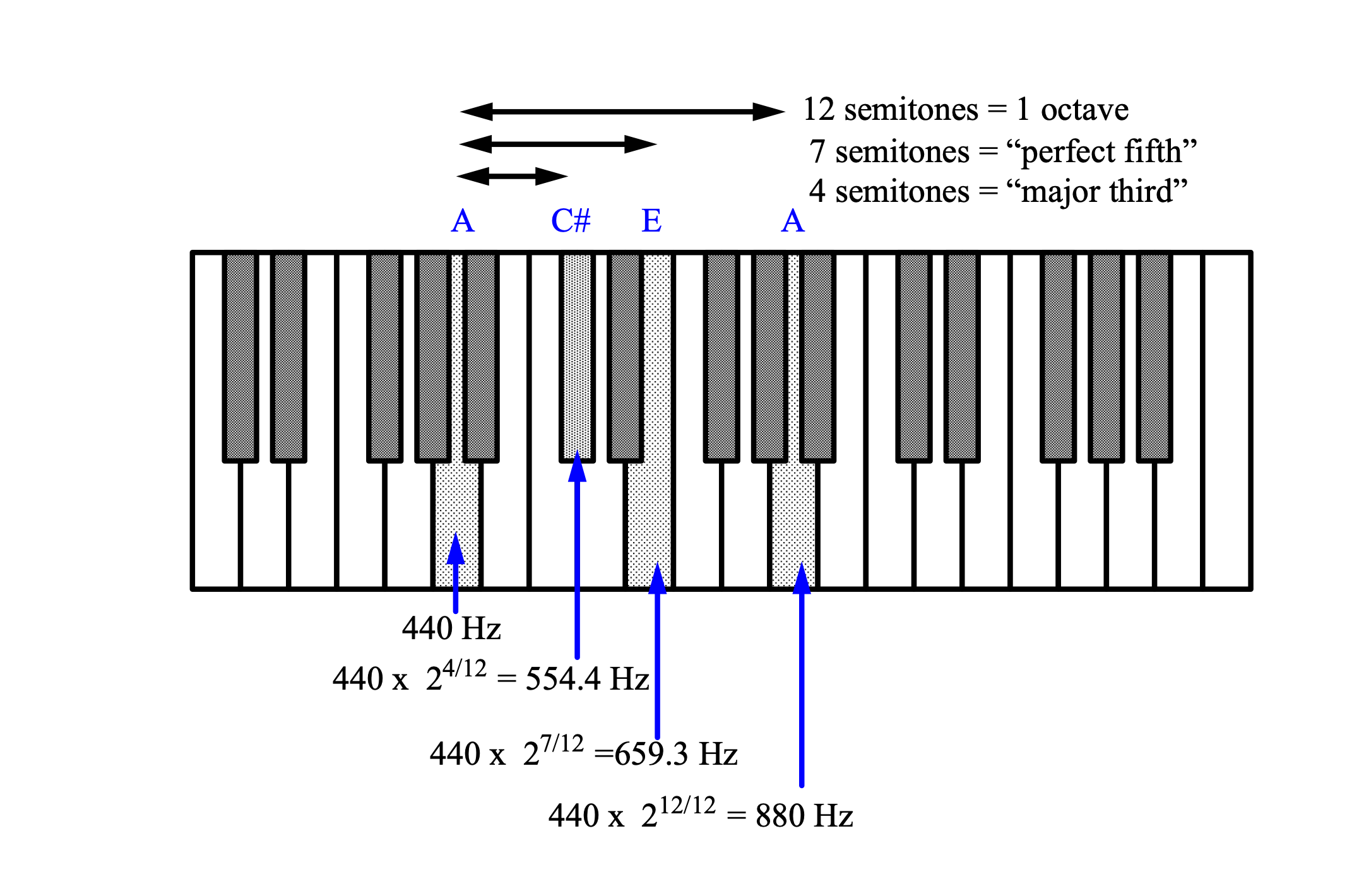
We can superimpose three tones to form a triad, or combine four :

Note the relationship between frequency and notes on the musical octave scale:

The spectrum

What is the frequency content of the signals that we’ve seen so far? In other words, what are the frequencies present in the signal? This is called the spectrum.

Let’s see a few examples

Pure tones or combinations of pure tones are fine, but they don’t sound very musical.

What are we missing? Harmonics!

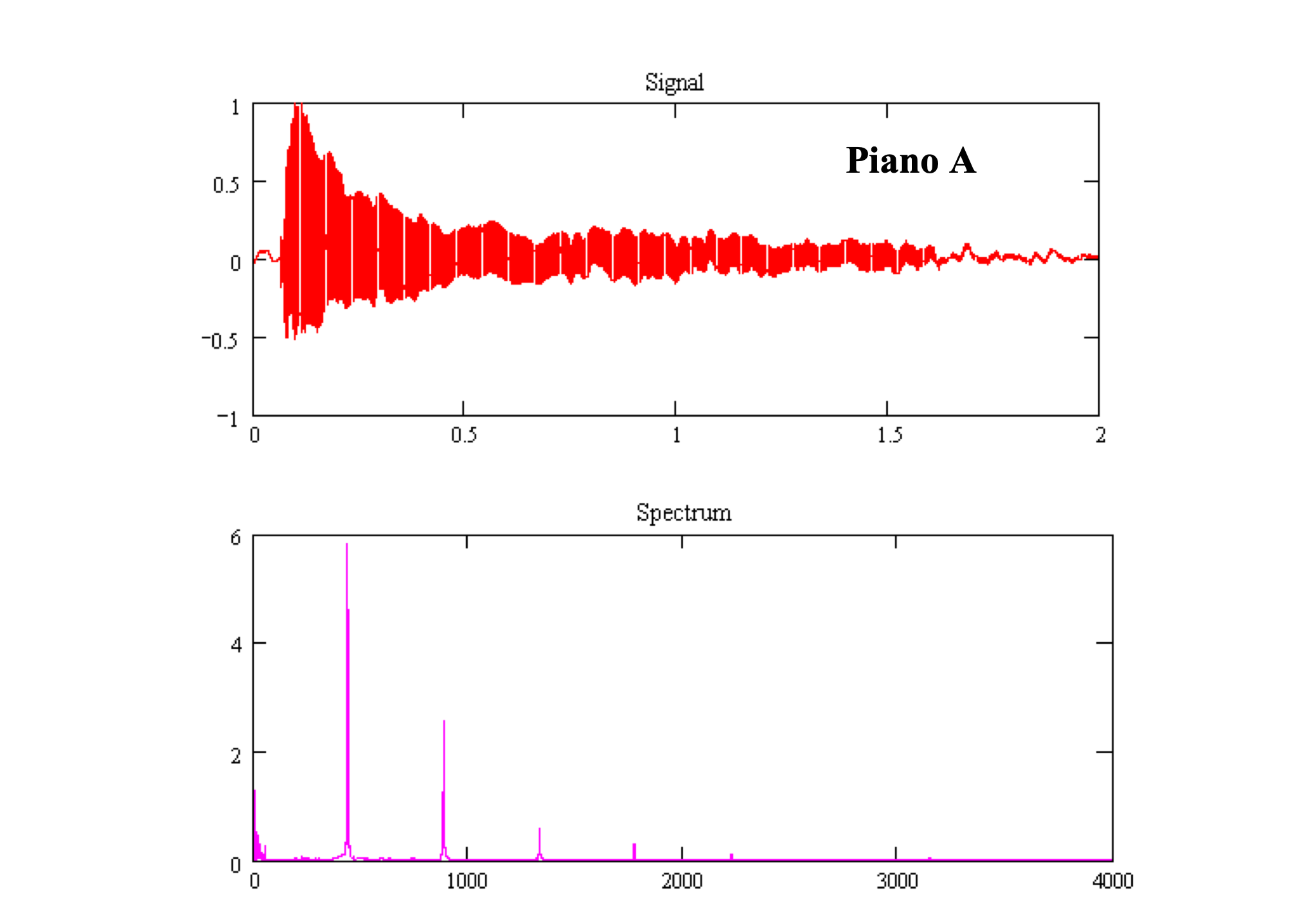
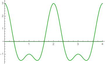
Musical instruments don’t play pure tones. They play periodic signals that are shaped by the characteristic of the instrument.

These periodic signals not only have a frequency spike at the fundamental frequency; they also have spikes at multiples of that frequency. These multiples, or overtones, correspond to the $2nd - nth$ harmonics of the instrument.

Different instruments weight these harmonics relatively differently to produce different sound.

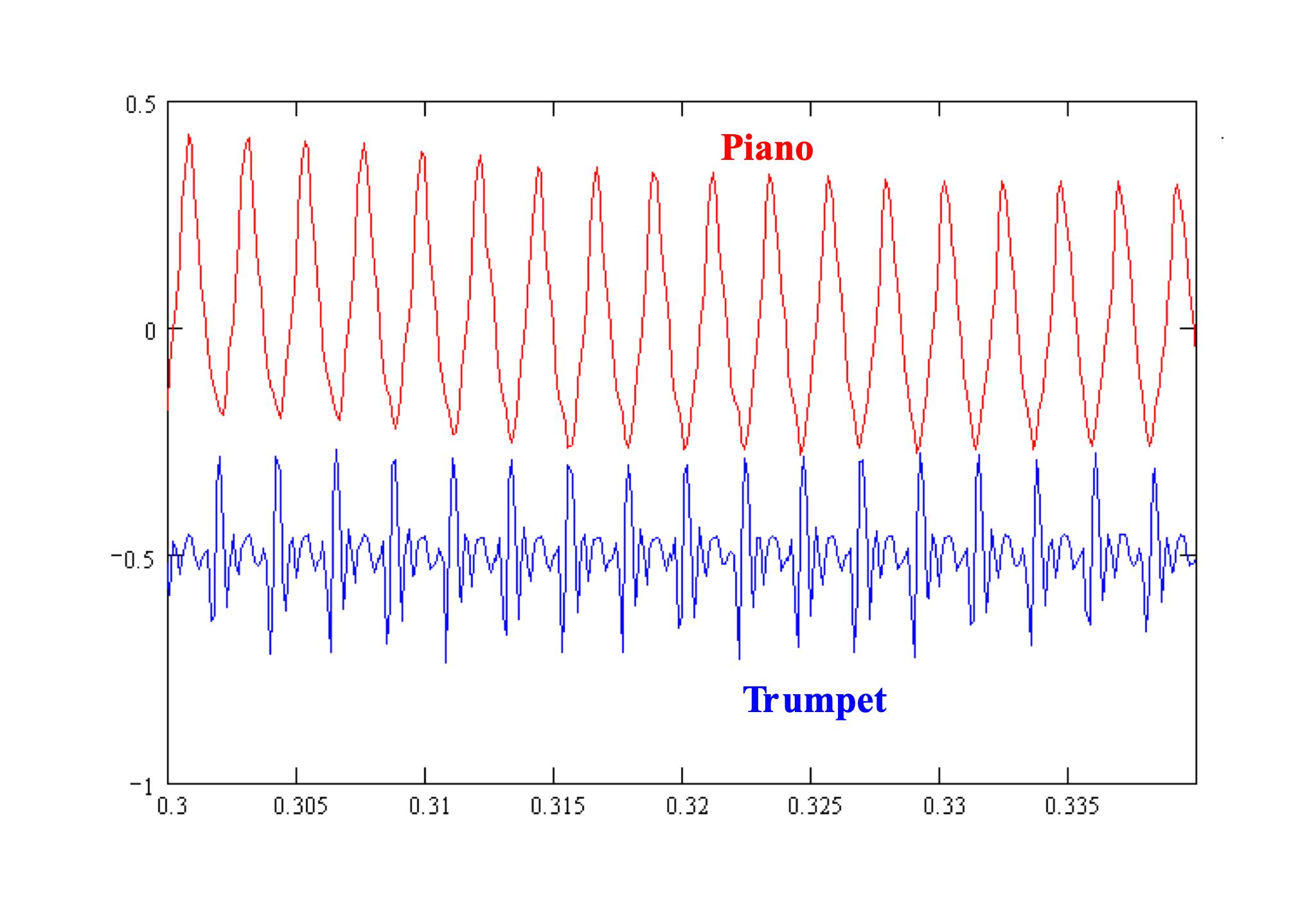
Piano

Trumpet

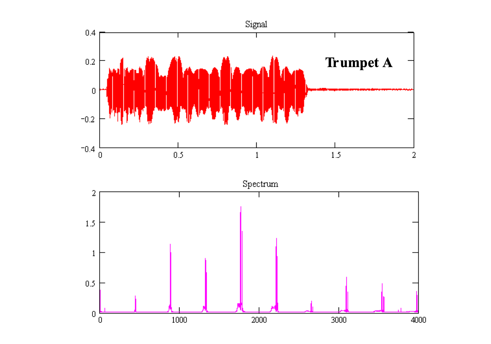
We see the same periodicity (high “A”) in the waveforms, but the character is different:

There’s a lot more that goes into the shape of a musical waveform and its impact on the corresponding sound. We won’t go into it in this class…

The “envelope” of the waveform: attack, sustain, and release

The timbre of the instrument: the texture created by the envelope and harmonic weightings

The underlying oscillation (cosine or some other waveform)

Loudness or volume

Tempo

Fourier series

Now that we have a general understanding of what frequency is, let’s see what’s actually going on.

We can write any periodic signal as a sum of sines and cosines!

$x\left( t \right) = a_{0} + \sum_{k = 1}^{\infty}\left( a_{k}\cos\left( \frac{2\pi kt}{T} \right) + b_{k}\sin\left( \frac{2\pi kt}{T} \right) \right)$

$a_{k}$ and $b_{k}$ tell us how much of each frequency is present

It turns out that it’s easier and more powerful to work with complex exponentials rather than sines and cosines. This is called the complex Fourier series:

$x\left( t \right) = \sum_{k = - \infty}^{\infty}{a_{k}e^{i2\pi kt/T}}$

Let’s take a closer look at For example,

$\color{green}{\cos\left( 2\pi ft \right)} = \color{blue}{\frac{1}{2}e^{i2\pi ft}} + \color{red}{\frac{1}{2}e^{- i2\pi ft}}$

Think of $\cos\left( 2\pi ft \right)$ as a point moving on the complex plane.

click on image to see more interesting examples

If the coefficient of $e^{i\omega t}$ and $e^{- i\omega t}$ are the same, the signal is real

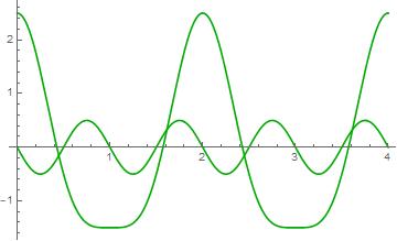
$\color{blue}{1e^{i2\pi 0.5t}} + \color{red}{1e^{- i2\pi 0.5t}} + \color{orange}{\frac{1}{2}e^{- i2\pi 1t}}$

$\color{blue}{1e^{i2\pi 0.5t}} + \color{red}{1e^{- i2\pi 0.5t}} + \color{purple}{\frac12e^{i2\pi1t}} + \color{orange}{\frac{1}{2}e^{- i2\pi 1t}}$

In addition to multiplying by nonnegative constants, we can change their starting angle by multiplying by terms of the form $e^{i\phi}$.

Fourier transform

But most functions are not periodic

Even the ones we talked about as periodic are bounded in time (do not repeat forever)

Instead of writing the frequency content as a sum, we write it as an integral

$x(t) = \int_{- \infty}^{\infty}{X\left( f \right)}e^{i2\pi ft}df$

Here, $X\left( f \right)$ determines “how much” of frequency $f$ is in signal $x(t)$

How do we find it? With this integral (we won’t be computing these integrals)

$X\left( f \right) = \int_{- \infty}^{\infty}{x\left( t \right)}e^{- i2\pi ft}dt$

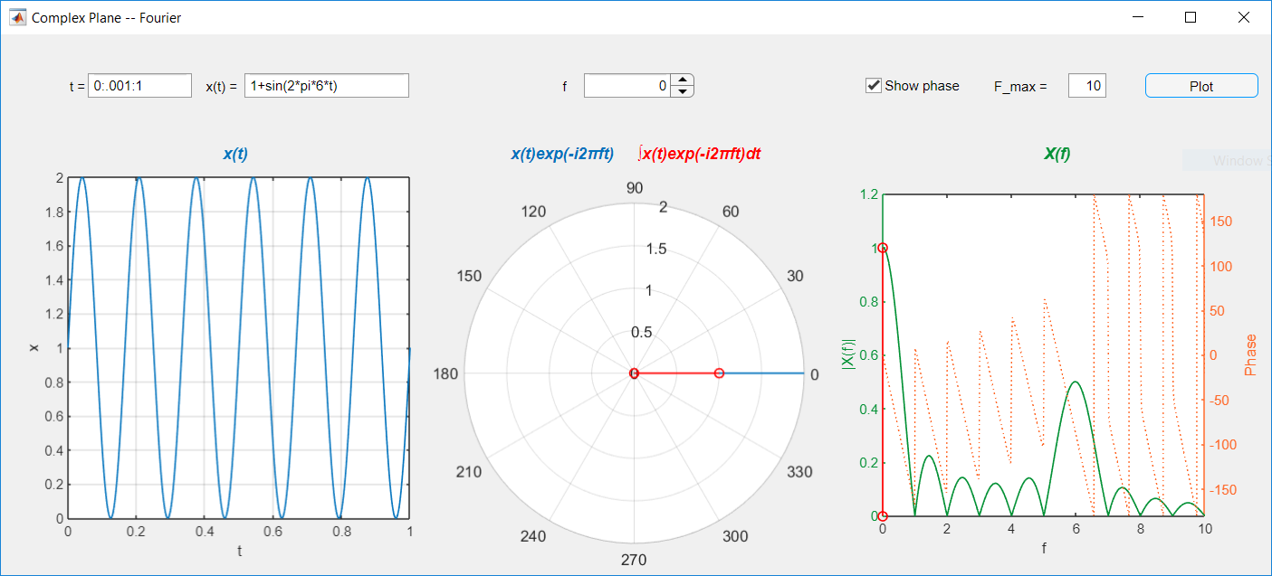
Finding $X(f)$ for a given $f$

Multiplying by $e^{- i2\pi ft}$ winds the signal around the origin in the complex plane. Each $1/f$ time units becomes one clockwise round around the origin.

The integral takes finds the average of the resulting curve.

The result is generally a complex number; we focus on $\vert X\left( f \right) \vert$

The Fourier transform of $1 + \sin\left( 2\pi 6t \right),0 \leq t \leq 1$ at $f = 0$ Hz

Stated differently: Every signal (video, audio, picture, etc.) has a frequency domain representation that is unique and contains all the information of the original signal. The way one computes the frequency domain representation from a given signal is called the Fourier transform.

We won’t worry about analytically computing Fourier transforms in this class – we’ll save that treat for ECE Fundamentals III ☺ Instead, we will focus on some important properties and let software like MATLAB plot spectra for us. Analytical equations are generally unavailable for real-world signals, anyway…

Important properties:

• Linearity
• Scaling time and frequency
• Symmetry
• Later: Multiplication by sinusoids, frequency response

Piano vs Trumpet, again Linearity

One observation from the previous examples: adding an A and a C# did not produce any “new” frequencies, just A, C# and harmonics. This is a consequence of the linearity. This property allows us to predict the spectrum of a combination of signals (e.g., a chord) from the spectra of the individual signals (e.g., pure tones). It can be divided into two elementary properties: Superposition: If x(t) has spectrum X(f), and y(t) has spectrum Y(f), then the sum x(t) + y(t) has the spectrum X(f) + Y(f). Scaling: If x(t) has spectrum X(f), and a is a constant, then, ax(t) has spectrum aX(f). Putting these together proves linearity: If x(t) has spectrum X(f), y(t) has spectrum Y(f), and a and b are both fixed, then ax(t) + by(t) has spectrum aX(f) + bY(f).

A more complex spectrum (just for fun)

Scaling time and frequency

The peak at 900 Hz is at 1800Hz if we double the speed If $X(f)$ is the spectrum of $x(t)$, then the spectrum of $x(at)$ is $X(\frac{f}a)$ Faster in time ($a>1$, graph shrinks) means higher frequencies (graph exapands) Conclusion: changing the speed of a musical recording changes pitch. To change speed without altering pitch is not straightforward!

*voice spinner in chrome music lab

High and low More examples Although complicated, there are distinct peaks. Can we determine the key from the spectrum? Major triad: B♭, D, F (B♭ is $440 \times 2^{1/12}$), Other peaks: notes in Bb major scale (C, E♭, G, A)

Another real-world spectrum Hallelujah chorus:

What do you notice about the predominant frequencies? Are all these frequencies being played at once?

Quantization error in the frequency domain

Symmetry

In general, given a complex-valued signal x(t), the spectrum X(f) has no guaranteed symmetry, and we need to look at both the positive and negative frequency axes to completely describe the signal. However, for a real-valued signal, the spectrum X(f) will have a special complex-valued symmetry called conjugate, or Hermitian, symmetry:

• The real component of the spectrum will have even symmetry: $X_R(f) = X_R(-f)$
• The imaginary component of the spectrum will have odd symmetry: $X_I(f) = -X_I(-f)$
• The magnitude of the spectrum will have even symmetry: $\vert X(f) \vert = \vert X(-f)\vert$
• The phase of the spectrum will have odd symmetry: $\angle X (f) = -\angle X(-f)$

Pure tones and frequency “spikes” Given a pure tone x(t) = cos(2πft), the frequency representation X(f) consists of a discontinuous spike at exactly ±f. More formally we call this spike a Dirac delta function δ(f-f0), centered at frequency f0. It has infinite height at frequency f0, and is zero at all other frequencies. Aside: In a strict mathematical sense, this function is undefined at f0. Instead, we define it implicitly, via the integral equationwhere X(f) is some real-valued function. Actually, even this definition is not strictly correct, but it’s close enough. The proper definition would require a graduate course in mathematical analysis. Setting X(f) = 1, we observe that the delta function has unit area.

Pure tones and frequency spikes

Note, we haven’t said anything about amplitude or phase here. This is because the spike’s location depends only on the sinusoid’s frequency. The amplitude A and phase φ will appear as a complex number Aeiφ multiplying the positive frequency (f0) spike and Ae-iφ multiplying the negative (-f0) spike.

In our plots before, we saw sinusoids that were limited in time. Their spectrum was similar to above, but not really a Dirac delta (we can’t really plot that with MATLAB)

Some Fourier transform examples

Frequency vs. time: the spectrogram

As we observed earlier, different sounds produce different frequency content. Music blends and varies different arrangements of these sounds through time. The Fourier spectrum provides a global picture of frequency content, it reflects all the frequencies present in the music. A more useful characterization of music would provide a local picture of frequency content as it varies through time. The spectrogram is one such characterization.

• spectrogram in chrome music lab

The spectrogram The spectrogram visualizes what we call the short-time Fourier transform. Normally, a single Fourier transform is computed for an entire signal. The short-time Fourier transform divides the signal into small, overlapping time intervals and computes a spectrum for each one separately. These spectra are plotted on a two-dimensional graph, with the frequency content along one axis, and the time dimension along the other. This 2D plot allows us to measure how the relative weighting of different frequency content changes through time. The spectrogram is one form of what is more generally called time-frequency analysis. Such methods allow engineers to design systems that analyze complicated signals in useful ways. Tools like Shazam form musical fingerprints from spectrograms to help identify music. Medical devices use time-frequency analysis to analyze heart rhythm.